Handling Tables in R

Author

Martin Schweinberger

Published

January 1, 2026

Introduction

This tutorial shows how to work with tables and how to process and manipulate tabular data in R. Tables are one of the most fundamental data structures in quantitative research: almost every dataset you will encounter — corpus metadata, survey responses, frequency counts, experimental results — arrives in tabular form. Knowing how to load, inspect, reshape, filter, summarise, join, and save tables efficiently is therefore one of the most important practical skills in R.

The tutorial uses the tidyverse family of packages throughout, particularly dplyr and tidyr. These packages provide a consistent, readable grammar for data manipulation that has become the standard in modern R programming. A highly recommended companion resource is Wickham and Grolemund (2016) (freely available at r4ds.had.co.nz), which covers these tools in much greater depth.

Prerequisite Tutorials

Before working through this tutorial, please complete or familiarise yourself with:

What This Tutorial Covers

Table types in R — matrices, data frames, and tibbles
Loading tables — CSV, TXT, Excel, and RDS formats
Inspecting tables — exploring structure, dimensions, and contents
Selecting and filtering — extracting columns and rows
Mutating and recoding — creating and modifying columns
Renaming and reordering — cleaning up column names
Sorting — arranging rows with arrange()
Grouping and summarising — collapsing data by group
Reshaping — pivoting between wide and long format
Joining tables — combining data from multiple sources
Handling missing values — detecting and dealing with NA
Saving tables — writing to CSV, Excel, and RDS

Citation

Martin Schweinberger. 2026. Handling Tables in R. The Language Technology and Data Analysis Laboratory (LADAL), The University of Queensland, Australia. url: https://ladal.edu.au/tutorials/table/table.html (Version 2026.03.28), doi: .

Preparation and Session Set-up

Install the required packages (once only):

Code

install.packages("dplyr")  
install.packages("tidyr")  
install.packages("flextable")  
install.packages("openxlsx")  
install.packages("readxl")  
install.packages("here")  
install.packages("checkdown")

Load the packages at the start of each session:

Code

library(dplyr)       # data manipulation  
library(tidyr)       # reshaping data  
library(flextable)   # formatted tables  
library(here)        # robust file paths  
library(checkdown)   # interactive exercises  
  
options(stringsAsFactors = FALSE)  
options(scipen = 100)  
options(max.print = 100)

We will use a simulated dataset throughout this tutorial. It represents a small corpus study: 120 observations of speech events from speakers across three registers, with metadata on speaker age, gender, proficiency, and word count.

Code

set.seed(42)  
  
corpus_meta <- data.frame(  
  doc_id      = paste0("doc", sprintf("%03d", 1:120)),  
  speaker_id  = paste0("spk", rep(1:40, each = 3)),  
  register    = rep(c("Academic", "News", "Fiction"), times = 40),  
  gender      = rep(c("Female", "Male", "Female", "Male",  
                      "Female", "Male", "Female", "Male",  
                      "Female", "Male"), each = 12),  
  age_group   = rep(c("18-30", "31-50", "51+"), times = 40),  
  l1          = sample(c("English", "German", "Mandarin", "Arabic"),  
                       120, replace = TRUE, prob = c(0.5, 0.2, 0.2, 0.1)),  
  word_count  = c(  
    round(rnorm(40, mean = 320, sd = 55)),   # Academic  
    round(rnorm(40, mean = 210, sd = 40)),   # News  
    round(rnorm(40, mean = 275, sd = 65))    # Fiction  
  ),  
  year        = sample(2018:2023, 120, replace = TRUE),  
  stringsAsFactors = FALSE  
)  
  
# Introduce a few missing values for later sections  
corpus_meta$word_count[c(5, 23, 67)] <- NA  
corpus_meta$l1[c(12, 88)] <- NA

We also create a second, smaller table that we will use for the joining section:

Code

speaker_info <- data.frame(  
  speaker_id    = paste0("spk", 1:40),  
  native_country = sample(  
    c("Australia", "UK", "Germany", "China", "Egypt"),  
    40, replace = TRUE, prob = c(0.35, 0.25, 0.2, 0.15, 0.05)  
  ),  
  education     = sample(c("Undergraduate", "Postgraduate", "PhD"),  
                         40, replace = TRUE),  
  stringsAsFactors = FALSE  
)

Table Types in R

Section Overview

What you’ll learn: The three main table types in R and when each is appropriate

Key concept: Data frames (and tibbles) are the standard for mixed-type tabular data

The three most common table types in R are:

Matrices store data of a single type only. If even one element is a character string, every other element is coerced to character as well. Matrices are used for numerical operations (e.g., in linear algebra or distance computations) but are rarely the right choice for storing research data with mixed variable types.

Data frames are the workhorse of R data analysis. Each column is a vector that can hold its own type (numeric, character, factor, logical), so different variable types coexist freely. Rows represent observations; columns represent variables.

Tibbles are the tidyverse version of data frames. They behave like data frames in almost all respects but have nicer default printing (they show only the first 10 rows and annotate column types), and they are slightly stricter about subsetting (less silent failure). All dplyr and tidyr operations work identically on data frames and tibbles.

Code

# A matrix: all values become character because of the name column
m <- matrix(c("Alice", "Bob", 28, 34), nrow = 2,
            dimnames = list(NULL, c("name", "age")))
class(m)

[1] "matrix" "array"

Code

typeof(m[1, "age"])   # character, not numeric!

[1] "character"

Code

# A data frame: types are preserved per column
df <- data.frame(name = c("Alice", "Bob"), age = c(28, 34))
class(df)

[1] "data.frame"

Code

class(df$age)               # numeric, as intended

[1] "numeric"

Code

# Convert a data frame to a tibble
tb <- tibble::as_tibble(df)
class(tb)

[1] "tbl_df"     "tbl"        "data.frame"

Which to Use?

Use data frames or tibbles for almost all research data — they preserve variable types and work seamlessly with all tidyverse functions. Use matrices only when you need to pass data to a function that specifically requires a matrix (e.g., dist(), hclust(), or matrix algebra).

Loading Tables into R

Section Overview

What you’ll learn: How to read tabular data from CSV, TXT, Excel, and RDS files

Key functions: read.csv(), read.delim(), readxl::read_excel(), readRDS()

CSV and TXT Files

Comma-separated values (CSV) files are the most portable format for tabular data. Use read.csv() for standard CSV files or read.delim() for tab-separated TXT files:

Code

# Load a CSV file  
mydata <- read.csv(here::here("data", "corpus_data.csv"))  
  
# Load a tab-separated TXT file  
mydata <- read.delim(here::here("data", "corpus_data.txt"),  
                     sep = "\t", header = TRUE)  
  
# Using read.table() — more flexible, more arguments to specify  
mydata <- read.table(here::here("data", "corpus_data.txt"),  
                     header = TRUE, sep = "\t", quote = "\"",  
                     stringsAsFactors = FALSE)

The tidyverse readr package provides faster alternatives with better default behaviour (no automatic factor conversion, cleaner column type detection):

Code

library(readr)  
mydata <- readr::read_csv(here::here("data", "corpus_data.csv"))  
mydata <- readr::read_tsv(here::here("data", "corpus_data.txt"))

Excel Files

Use readxl::read_excel() to load Excel workbooks. This package is part of the tidyverse and requires no installation if you have already installed tidyverse:

Code

library(readxl)  
  
# Load the first sheet  
mydata <- readxl::read_excel(here::here("data", "corpus_data.xlsx"),  
                              sheet = 1)  
  
# Load by sheet name  
mydata <- readxl::read_excel(here::here("data", "corpus_data.xlsx"),  
                              sheet = "Sheet2")  
  
# Load only specific rows and columns  
mydata <- readxl::read_excel(here::here("data", "corpus_data.xlsx"),  
                              range = "A1:F50")

The openxlsx package is useful when you also need to write formatted Excel files (see the Saving Tables section):

Code

library(openxlsx)  
mydata <- openxlsx::read.xlsx(here::here("data", "corpus_data.xlsx"),  
                               sheet = 1)

RDS Files

R’s native binary format (.rds) preserves all R-specific attributes — factor levels, column types, and so on — exactly as they were when saved. It is the best format for saving and reloading data between R sessions:

Code

# Load an RDS file  
mydata <- readRDS(here::here("data", "corpus_data.rds"))

Using here::here() for File Paths

Always use here::here() rather than hardcoded absolute paths ("C:/Users/Martin/...") or relative paths that depend on your working directory. here() constructs paths relative to the root of your R Project, so code works identically on any computer. See the Getting Started tutorial for how to set up an R Project.

Inspecting Tables

Section Overview

What you’ll learn: How to quickly understand the shape, structure, and content of a table

Key functions: head(), tail(), str(), glimpse(), summary(), dim(), names()

Before doing anything with a dataset, always inspect it first. A handful of functions give you a rapid, comprehensive picture.

Code

# First 6 rows (default)  
head(corpus_meta)

  doc_id speaker_id register gender age_group       l1 word_count year
1 doc001       spk1 Academic Female     18-30   Arabic        300 2018
2 doc002       spk1     News Female     31-50   Arabic        330 2020
3 doc003       spk1  Fiction Female       51+  English        352 2020
4 doc004       spk2 Academic Female     18-30   German        397 2021
5 doc005       spk2     News Female     31-50 Mandarin         NA 2022
6 doc006       spk2  Fiction Female       51+ Mandarin        392 2021

Code

# First 10 rows  
head(corpus_meta, 10)

   doc_id speaker_id register gender age_group       l1 word_count year
1  doc001       spk1 Academic Female     18-30   Arabic        300 2018
2  doc002       spk1     News Female     31-50   Arabic        330 2020
3  doc003       spk1  Fiction Female       51+  English        352 2020
4  doc004       spk2 Academic Female     18-30   German        397 2021
5  doc005       spk2     News Female     31-50 Mandarin         NA 2022
6  doc006       spk2  Fiction Female       51+ Mandarin        392 2021
7  doc007       spk3 Academic Female     18-30   German        338 2019
8  doc008       spk3     News Female     31-50  English        377 2023
9  doc009       spk3  Fiction Female       51+ Mandarin        371 2018
10 doc010       spk4 Academic Female     18-30   German        360 2023

Code

# Last 6 rows  
tail(corpus_meta)

    doc_id speaker_id register gender age_group       l1 word_count year
115 doc115      spk39 Academic   Male     18-30 Mandarin        331 2021
116 doc116      spk39     News   Male     31-50 Mandarin        265 2018
117 doc117      spk39  Fiction   Male       51+  English        181 2023
118 doc118      spk40 Academic   Male     18-30  English        317 2019
119 doc119      spk40     News   Male     31-50 Mandarin        306 2020
120 doc120      spk40  Fiction   Male       51+   German        275 2018

Code

# Dimensions (rows × columns)  
dim(corpus_meta)

[1] 120   8

Code

nrow(corpus_meta)

[1] 120

Code

ncol(corpus_meta)

[1] 8

Code

# Column names  
names(corpus_meta)

[1] "doc_id"     "speaker_id" "register"   "gender"     "age_group" 
[6] "l1"         "word_count" "year"

Code

# Structure: column types and first values  
str(corpus_meta)

'data.frame':   120 obs. of  8 variables:
 $ doc_id    : chr  "doc001" "doc002" "doc003" "doc004" ...
 $ speaker_id: chr  "spk1" "spk1" "spk1" "spk2" ...
 $ register  : chr  "Academic" "News" "Fiction" "Academic" ...
 $ gender    : chr  "Female" "Female" "Female" "Female" ...
 $ age_group : chr  "18-30" "31-50" "51+" "18-30" ...
 $ l1        : chr  "Arabic" "Arabic" "English" "German" ...
 $ word_count: num  300 330 352 397 NA 392 338 377 371 360 ...
 $ year      : int  2018 2020 2020 2021 2022 2021 2019 2023 2018 2023 ...

Code

# tidyverse-style structure overview (more readable)  
dplyr::glimpse(corpus_meta)

Rows: 120
Columns: 8
$ doc_id     <chr> "doc001", "doc002", "doc003", "doc004", "doc005", "doc006",…
$ speaker_id <chr> "spk1", "spk1", "spk1", "spk2", "spk2", "spk2", "spk3", "sp…
$ register   <chr> "Academic", "News", "Fiction", "Academic", "News", "Fiction…
$ gender     <chr> "Female", "Female", "Female", "Female", "Female", "Female",…
$ age_group  <chr> "18-30", "31-50", "51+", "18-30", "31-50", "51+", "18-30", …
$ l1         <chr> "Arabic", "Arabic", "English", "German", "Mandarin", "Manda…
$ word_count <dbl> 300, 330, 352, 397, NA, 392, 338, 377, 371, 360, 263, 315, …
$ year       <int> 2018, 2020, 2020, 2021, 2022, 2021, 2019, 2023, 2018, 2023,…

Code

# Statistical summary per column  
summary(corpus_meta)

    doc_id           speaker_id          register            gender         
 Length:120         Length:120         Length:120         Length:120        
 Class :character   Class :character   Class :character   Class :character  
 Mode  :character   Mode  :character   Mode  :character   Mode  :character  
                                                                            
                                                                            
                                                                            
                                                                            
  age_group              l1              word_count         year     
 Length:120         Length:120         Min.   :129.0   Min.   :2018  
 Class :character   Class :character   1st Qu.:210.0   1st Qu.:2019  
 Mode  :character   Mode  :character   Median :260.0   Median :2020  
                                       Mean   :267.4   Mean   :2020  
                                       3rd Qu.:324.0   3rd Qu.:2022  
                                       Max.   :403.0   Max.   :2023  
                                       NA's   :3

The summary() output is especially useful: it shows the range, quartiles, and mean for numeric columns, and a frequency table for factor columns. Crucially, it also shows the count of NA values per column — a quick way to spot missing data.

Exercises: Inspecting Tables

Q1. You receive a new dataset and run dim(df) which returns c(2500, 18). What does this tell you?

Q2. Which function provides the most compact overview of column names AND their types AND the first few values in one call?

Selecting and Filtering

Section Overview

What you’ll learn: How to extract specific columns and rows from a data frame

Key functions: dplyr::select(), dplyr::filter()

Key concept: select() operates on columns; filter() operates on rows

Selecting Columns with `select()`

select() keeps only the columns you name. It never changes the rows.

Code

# Keep specific columns by name  
corpus_meta |>  
  dplyr::select(doc_id, register, word_count) |>  
  head(5)

  doc_id register word_count
1 doc001 Academic        300
2 doc002     News        330
3 doc003  Fiction        352
4 doc004 Academic        397
5 doc005     News         NA

Code

# Remove a column with -  
corpus_meta |>  
  dplyr::select(-year, -l1) |>  
  head(5)

  doc_id speaker_id register gender age_group word_count
1 doc001       spk1 Academic Female     18-30        300
2 doc002       spk1     News Female     31-50        330
3 doc003       spk1  Fiction Female       51+        352
4 doc004       spk2 Academic Female     18-30        397
5 doc005       spk2     News Female     31-50         NA

select() also accepts helper functions that select columns by pattern, type, or position:

Code

# Columns whose names start with a given string  
corpus_meta |>  
  dplyr::select(dplyr::starts_with("s")) |>  
  head(3)

  speaker_id
1       spk1
2       spk1
3       spk1

Code

# Columns whose names contain a given string  
corpus_meta |>  
  dplyr::select(dplyr::contains("_id")) |>  
  head(3)

  doc_id speaker_id
1 doc001       spk1
2 doc002       spk1
3 doc003       spk1

Code

# Select and rename in one step  
corpus_meta |>  
  dplyr::select(Document = doc_id, Register = register, Words = word_count) |>  
  head(3)

  Document Register Words
1   doc001 Academic   300
2   doc002     News   330
3   doc003  Fiction   352

Filtering Rows with `filter()`

filter() keeps only rows where the condition is TRUE. It never changes the columns.

Code

# Keep only Academic texts  
corpus_meta |>  
  dplyr::filter(register == "Academic") |>  
  nrow()

[1] 40

Code

# Multiple conditions: Academic texts with more than 300 words  
corpus_meta |>  
  dplyr::filter(register == "Academic", word_count > 300) |>  
  head(5)

  doc_id speaker_id register gender age_group     l1 word_count year
1 doc004       spk2 Academic Female     18-30 German        397 2021
2 doc007       spk3 Academic Female     18-30 German        338 2019
3 doc010       spk4 Academic Female     18-30 German        360 2023
4 doc013       spk5 Academic   Male     18-30 Arabic        354 2023
5 doc016       spk6 Academic   Male     18-30 Arabic        352 2021

Code

# OR condition: Academic OR Fiction  
corpus_meta |>  
  dplyr::filter(register %in% c("Academic", "Fiction")) |>  
  dplyr::count(register)

  register  n
1 Academic 40
2  Fiction 40

Code

# Filter on a partial string match  
corpus_meta |>  
  dplyr::filter(stringr::str_detect(doc_id, "00[12]$")) |>  
  head(5)

  doc_id speaker_id register gender age_group     l1 word_count year
1 doc001       spk1 Academic Female     18-30 Arabic        300 2018
2 doc002       spk1     News Female     31-50 Arabic        330 2020

Combining select() and filter()

The two functions are almost always used together in a pipeline: first filter the rows you need, then select the columns you need:

Code

corpus_meta |>  
  dplyr::filter(gender == "Female", age_group == "18-30") |>  
  dplyr::select(doc_id, register, word_count) |>  
  head(5)

  doc_id register word_count
1 doc001 Academic        300
2 doc004 Academic        397
3 doc007 Academic        338
4 doc010 Academic        360
5 doc025 Academic        254

Exercises: Selecting and Filtering

Q1. What is the key difference between select() and filter()?

Q2. You want to keep only rows where register is \"News\" AND word_count is greater than 200. Which code is correct?

Mutating and Recoding

Section Overview

What you’ll learn: How to create new columns and modify existing ones

Key functions: dplyr::mutate(), dplyr::if_else(), dplyr::case_when()

mutate() adds new columns or overwrites existing ones while keeping all rows and all other columns unchanged.

Adding a New Column

Code

# Add a column for word count in thousands  
corpus_meta <- corpus_meta |>  
  dplyr::mutate(word_count_k = round(word_count / 1000, 3))  
  
head(corpus_meta[, c("doc_id", "word_count", "word_count_k")], 5)

  doc_id word_count word_count_k
1 doc001        300        0.300
2 doc002        330        0.330
3 doc003        352        0.352
4 doc004        397        0.397
5 doc005         NA           NA

Binary Recoding with `if_else()`

Use dplyr::if_else() (the type-safe tidyverse version of base R ifelse()) to recode a column into two categories:

Code

corpus_meta <- corpus_meta |>  
  dplyr::mutate(  
    length_class = dplyr::if_else(word_count >= 300, "Long", "Short")  
  )  
  
table(corpus_meta$length_class, useNA = "ifany")


 Long Short  <NA> 
   41    76     3

Multi-Category Recoding with `case_when()`

case_when() is the tidyverse equivalent of a chain of if/else if statements. Conditions are evaluated top-to-bottom and the first match wins. The final TRUE ~ acts as the catch-all default:

Code

corpus_meta <- corpus_meta |>  
  dplyr::mutate(  
    length_band = dplyr::case_when(  
      word_count <  200              ~ "Very short",  
      word_count >= 200 & word_count < 300 ~ "Short",  
      word_count >= 300 & word_count < 400 ~ "Long",  
      word_count >= 400              ~ "Very long",  
      TRUE                           ~ NA_character_   # catches NA word counts  
    )  
  )  
  
table(corpus_meta$length_band, useNA = "ifany")


      Long      Short  Very long Very short       <NA> 
        40         54          1         22          3

Recoding Based on String Patterns

Combine mutate() with stringr::str_detect() to recode based on partial string matches — a pattern that comes up constantly in corpus linguistics when working with file names or speaker IDs:

Code

corpus_meta <- corpus_meta |>  
  dplyr::mutate(  
    period = dplyr::case_when(  
      year %in% 2018:2019 ~ "Early",  
      year %in% 2020:2021 ~ "Mid",  
      year %in% 2022:2023 ~ "Recent",  
      TRUE                ~ "Unknown"  
    )  
  )  
  
table(corpus_meta$period)


 Early    Mid Recent 
    41     41     38

Modifying an Existing Column

Use the same column name on the left-hand side of mutate() to overwrite an existing column:

Code

# Convert register to a factor with a custom level order  
corpus_meta <- corpus_meta |>  
  dplyr::mutate(  
    register = factor(register,  
                      levels = c("Academic", "News", "Fiction"))  
  )  
  
levels(corpus_meta$register)

[1] "Academic" "News"     "Fiction"

Exercises: Mutating

Q1. What happens if you use the same column name on both sides of mutate()?

Q2. In a case_when() call, what happens to rows that do not match any condition and there is no TRUE ~ catch-all?

Renaming and Reordering Columns

Section Overview

What you’ll learn: How to rename columns and change their order

Key functions: dplyr::rename(), dplyr::relocate()

Renaming with `rename()`

rename() uses new_name = old_name syntax:

Code

corpus_renamed <- corpus_meta |>  
  dplyr::rename(  
    Document  = doc_id,  
    Speaker   = speaker_id,  
    Register  = register,  
    Gender    = gender,  
    AgeGroup  = age_group,  
    L1        = l1,  
    WordCount = word_count,  
    Year      = year  
  )  
  
names(corpus_renamed)

 [1] "Document"     "Speaker"      "Register"     "Gender"       "AgeGroup"    
 [6] "L1"           "WordCount"    "Year"         "word_count_k" "length_class"
[11] "length_band"  "period"

Renaming by Pattern with `rename_with()`

rename_with() applies a function to column names — useful for bulk transformations:

Code

# Capitalise the first letter of every column name  
corpus_meta |>  
  dplyr::rename_with(stringr::str_to_title) |>  
  names()

 [1] "Doc_id"       "Speaker_id"   "Register"     "Gender"       "Age_group"   
 [6] "L1"           "Word_count"   "Year"         "Word_count_k" "Length_class"
[11] "Length_band"  "Period"

Code

# Replace all underscores with dots  
corpus_meta |>  
  dplyr::rename_with(~ gsub("_", ".", .x)) |>  
  names()

 [1] "doc.id"       "speaker.id"   "register"     "gender"       "age.group"   
 [6] "l1"           "word.count"   "year"         "word.count.k" "length.class"
[11] "length.band"  "period"

Reordering Columns with `relocate()`

relocate() moves columns to a new position without dropping any:

Code

# Move word_count to the front  
corpus_meta |>  
  dplyr::relocate(word_count, .before = doc_id) |>  
  head(3)

  word_count doc_id speaker_id register gender age_group      l1 year
1        300 doc001       spk1 Academic Female     18-30  Arabic 2018
2        330 doc002       spk1     News Female     31-50  Arabic 2020
3        352 doc003       spk1  Fiction Female       51+ English 2020
  word_count_k length_class length_band period
1        0.300         Long        Long  Early
2        0.330         Long        Long    Mid
3        0.352         Long        Long    Mid

Code

# Move year and l1 to after register  
corpus_meta |>  
  dplyr::relocate(year, l1, .after = register) |>  
  head(3)

  doc_id speaker_id register year      l1 gender age_group word_count
1 doc001       spk1 Academic 2018  Arabic Female     18-30        300
2 doc002       spk1     News 2020  Arabic Female     31-50        330
3 doc003       spk1  Fiction 2020 English Female       51+        352
  word_count_k length_class length_band period
1        0.300         Long        Long  Early
2        0.330         Long        Long    Mid
3        0.352         Long        Long    Mid

Sorting with `arrange()`

Section Overview

What you’ll learn: How to sort rows in ascending or descending order, including multi-column sorting

Key function: dplyr::arrange()

arrange() sorts rows by one or more columns. The default is ascending order; wrap a column in desc() for descending:

Code

# Sort by word count, ascending (shortest first)  
corpus_meta |>  
  dplyr::select(doc_id, register, word_count) |>  
  dplyr::arrange(word_count) |>  
  head(8)

  doc_id register word_count
1 doc068     News        129
2 doc055 Academic        144
3 doc061 Academic        150
4 doc062     News        151
5 doc059     News        156
6 doc069  Fiction        161
7 doc113     News        162
8 doc076 Academic        166

Code

# Sort by word count, descending (longest first)  
corpus_meta |>  
  dplyr::select(doc_id, register, word_count) |>  
  dplyr::arrange(dplyr::desc(word_count)) |>  
  head(8)

  doc_id register word_count
1 doc021  Fiction        403
2 doc004 Academic        397
3 doc031 Academic        397
4 doc034 Academic        397
5 doc006  Fiction        392
6 doc114  Fiction        385
7 doc008     News        377
8 doc009  Fiction        371

Code

# Multi-column sort: register (alphabetical), then word_count (descending)  
corpus_meta |>  
  dplyr::select(doc_id, register, word_count) |>  
  dplyr::arrange(register, dplyr::desc(word_count)) |>  
  head(10)

   doc_id register word_count
1  doc004 Academic        397
2  doc031 Academic        397
3  doc034 Academic        397
4  doc106 Academic        368
5  doc010 Academic        360
6  doc100 Academic        359
7  doc040 Academic        356
8  doc013 Academic        354
9  doc016 Academic        352
10 doc007 Academic        338

NA Values in arrange()

Missing values are always sorted to the end by arrange(), regardless of ascending or descending order. Use dplyr::filter(!is.na(column)) before arrange() if you want to exclude them first.

Grouping and Summarising

Section Overview

What you’ll learn: How to compute group-level summaries — the most common operation in descriptive data analysis

Key functions: dplyr::group_by(), dplyr::summarise(), dplyr::count()

group_by() splits the data into groups; summarise() computes summary statistics within each group and collapses rows to one per group.

Basic Group Summary

Code

corpus_meta |>  
  dplyr::group_by(register) |>  
  dplyr::summarise(  
    n         = dplyr::n(),  
    mean_wc   = round(mean(word_count, na.rm = TRUE), 1),  
    sd_wc     = round(sd(word_count, na.rm = TRUE), 1),  
    min_wc    = min(word_count, na.rm = TRUE),  
    max_wc    = max(word_count, na.rm = TRUE),  
    .groups   = "drop"  
  ) |>  
  flextable() |>  
  flextable::set_table_properties(width = .75, layout = "autofit") |>  
  flextable::theme_zebra() |>  
  flextable::fontsize(size = 12) |>  
  flextable::fontsize(size = 12, part = "header") |>  
  flextable::align_text_col(align = "center") |>  
  flextable::set_caption(caption = "Word count summary by register.") |>  
  flextable::border_outer()

register	n	mean_wc	sd_wc	min_wc	max_wc
Academic	40	278.1	73.1	144	397
News	40	252.8	64.7	129	377
Fiction	40	271.0	69.0	161	403

Multi-Variable Grouping

Code

corpus_meta |>  
  dplyr::group_by(register, gender) |>  
  dplyr::summarise(  
    n       = dplyr::n(),  
    mean_wc = round(mean(word_count, na.rm = TRUE), 1),  
    .groups = "drop"  
  ) |>  
  flextable() |>  
  flextable::set_table_properties(width = .6, layout = "autofit") |>  
  flextable::theme_zebra() |>  
  flextable::fontsize(size = 12) |>  
  flextable::fontsize(size = 12, part = "header") |>  
  flextable::align_text_col(align = "center") |>  
  flextable::set_caption(caption = "Word count by register and gender.") |>  
  flextable::border_outer()

register	gender	n	mean_wc
Academic	Female	20	285.9
Academic	Male	20	269.9
News	Female	20	256.2
News	Male	20	249.5
Fiction	Female	20	283.3
Fiction	Male	20	258.6

`count()` — Quick Frequency Tables

count() is a shortcut for group_by() + summarise(n = n()):

Code

# Frequency of each register  
corpus_meta |>  
  dplyr::count(register)

  register  n
1 Academic 40
2     News 40
3  Fiction 40

Code

# Cross-tabulation: register × gender  
corpus_meta |>  
  dplyr::count(register, gender)

  register gender  n
1 Academic Female 20
2 Academic   Male 20
3     News Female 20
4     News   Male 20
5  Fiction Female 20
6  Fiction   Male 20

Code

# Sort by frequency  
corpus_meta |>  
  dplyr::count(l1, sort = TRUE)

        l1  n
1  English 51
2 Mandarin 27
3   German 22
4   Arabic 18
5     <NA>  2

`mutate()` After `group_by()`

When mutate() follows group_by(), it computes the new column within each group but retains all original rows — useful for computing group means alongside individual values:

Code

corpus_meta |>  
  dplyr::group_by(register) |>  
  dplyr::mutate(  
    group_mean_wc = round(mean(word_count, na.rm = TRUE), 1),  
    deviation     = word_count - group_mean_wc  
  ) |>  
  dplyr::ungroup() |>  
  dplyr::select(doc_id, register, word_count, group_mean_wc, deviation) |>  
  head(8)

# A tibble: 8 × 5
  doc_id register word_count group_mean_wc deviation
  <chr>  <fct>         <dbl>         <dbl>     <dbl>
1 doc001 Academic        300          278.      21.9
2 doc002 News            330          253.      77.2
3 doc003 Fiction         352          271       81  
4 doc004 Academic        397          278.     119. 
5 doc005 News             NA          253.      NA  
6 doc006 Fiction         392          271      121  
7 doc007 Academic        338          278.      59.9
8 doc008 News            377          253.     124.

Always ungroup() After group_by()

After using group_by(), the data frame remains “grouped” until you explicitly ungroup() it. Grouped data frames can produce unexpected results in subsequent operations. Always add dplyr::ungroup() at the end of any pipeline that uses group_by(), or use the .groups = "drop" argument inside summarise().

Exercises: Summarising

Q1. What is the key difference between using mutate() and summarise() after group_by()?

Q2. What does .groups = \"drop\" do inside summarise()?

Reshaping: Wide and Long Format

Section Overview

What you’ll learn: How to convert data between wide format and long format using pivot_longer() and pivot_wider()

Key concept: Long format has one row per observation; wide format has one row per subject with multiple measurement columns

Note on older functions: The tidyverse functions gather() and spread() are deprecated and replaced by pivot_longer() and pivot_wider(). This tutorial uses the modern versions.

Reshaping is one of the most frequently needed — and most frequently confusing — data operations. The key is understanding the two formats:

Wide format: Each subject occupies one row; repeated measurements are spread across multiple columns (e.g., score_time1, score_time2, score_time3). Easy for humans to read; needed for some statistical functions.

Long format: Each measurement is its own row; a column identifies which measurement it is. Required by ggplot2 and most tidy statistical functions.

Let us create a small wide-format summary to demonstrate:

Code

# Create a wide-format summary: mean word count per register × gender  
wide_summary <- corpus_meta |>  
  dplyr::group_by(register, gender) |>  
  dplyr::summarise(mean_wc = round(mean(word_count, na.rm = TRUE), 1),  
                   .groups = "drop") |>  
  tidyr::pivot_wider(names_from = gender, values_from = mean_wc)  
  
wide_summary |>  
  flextable() |>  
  flextable::set_table_properties(width = .5, layout = "autofit") |>  
  flextable::theme_zebra() |>  
  flextable::fontsize(size = 12) |>  
  flextable::fontsize(size = 12, part = "header") |>  
  flextable::align_text_col(align = "center") |>  
  flextable::set_caption(caption = "Mean word count per register × gender (wide format).") |>  
  flextable::border_outer()

register	Female	Male
Academic	285.9	269.9
News	256.2	249.5
Fiction	283.3	258.6

Wide to Long: `pivot_longer()`

pivot_longer() gathers multiple columns into key-value pairs — it makes the data longer (more rows, fewer columns):

Code

long_summary <- wide_summary |>  
  tidyr::pivot_longer(  
    cols      = c(Female, Male),   # columns to gather  
    names_to  = "gender",          # new column for the old column names  
    values_to = "mean_wc"          # new column for the values  
  )  
  
long_summary

# A tibble: 6 × 3
  register gender mean_wc
  <fct>    <chr>    <dbl>
1 Academic Female    286.
2 Academic Male      270.
3 News     Female    256.
4 News     Male      250.
5 Fiction  Female    283.
6 Fiction  Male      259.

Long to Wide: `pivot_wider()`

pivot_wider() spreads a key-value pair across multiple columns — it makes the data wider (fewer rows, more columns):

Code

# Back to wide format  
long_summary |>  
  tidyr::pivot_wider(  
    names_from  = gender,    # column whose values become new column names  
    values_from = mean_wc    # column whose values fill the new columns  
  )

# A tibble: 3 × 3
  register Female  Male
  <fct>     <dbl> <dbl>
1 Academic   286.  270.
2 News       256.  250.
3 Fiction    283.  259.

A Linguistic Example

A common situation in corpus work: you have measurements for several linguistic features across multiple text types, and you need to switch between formats depending on whether you are computing a table (wide) or a plot (long):

Code

# Simulate feature counts per register  
features_wide <- data.frame(  
  register       = c("Academic", "News", "Fiction"),  
  passive_rate   = c(0.12, 0.06, 0.03),  
  nominalisation = c(0.18, 0.09, 0.05),  
  hedging        = c(0.08, 0.04, 0.11)  
)  
  
# Convert to long format for plotting  
features_long <- features_wide |>  
  tidyr::pivot_longer(  
    cols      = -register,         # all columns except register  
    names_to  = "feature",  
    values_to = "rate"  
  )  
  
features_long

# A tibble: 9 × 3
  register feature         rate
  <chr>    <chr>          <dbl>
1 Academic passive_rate    0.12
2 Academic nominalisation  0.18
3 Academic hedging         0.08
4 News     passive_rate    0.06
5 News     nominalisation  0.09
6 News     hedging         0.04
7 Fiction  passive_rate    0.03
8 Fiction  nominalisation  0.05
9 Fiction  hedging         0.11

Code

# Plot in long format  
ggplot2::ggplot(features_long,  
                ggplot2::aes(x = register, y = rate, fill = register)) +  
  ggplot2::geom_col() +  
  ggplot2::facet_wrap(~ feature) +  
  ggplot2::scale_fill_manual(values = c("steelblue", "tomato", "seagreen")) +  
  ggplot2::theme_bw() +  
  ggplot2::theme(legend.position = "none",  
                 panel.grid.minor = ggplot2::element_blank()) +  
  ggplot2::labs(title = "Linguistic feature rates by register",  
                x = "Register", y = "Rate")

Exercises: Reshaping

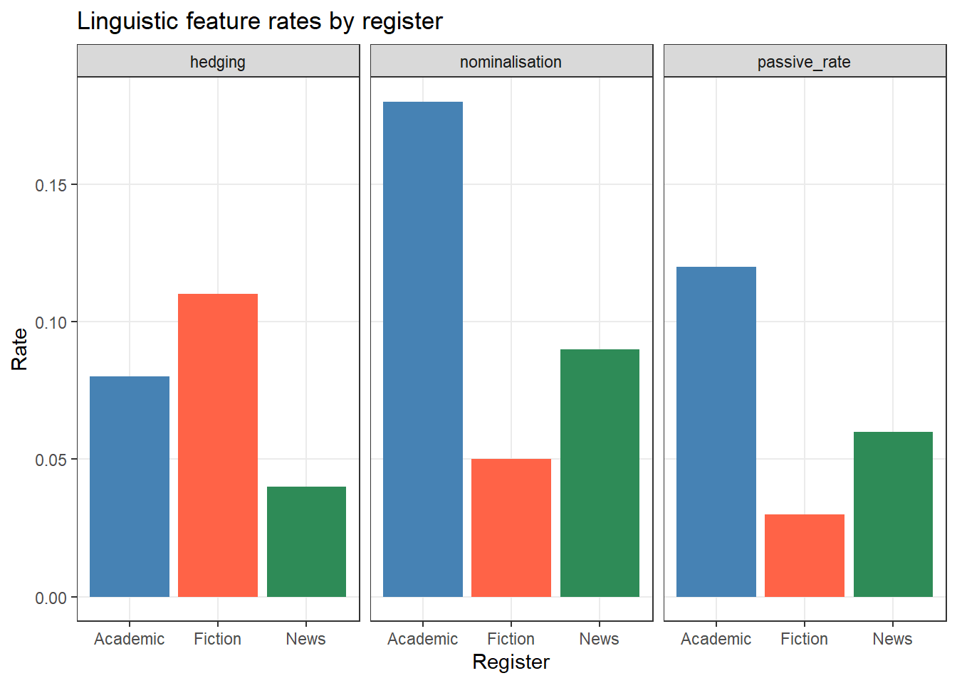
Q1. Which format does ggplot2 require for plotting grouped data?

Q2. What is the modern tidyverse replacement for the deprecated gather() and spread() functions?

Joining Tables

Section Overview

What you’ll learn: How to combine two data frames by matching on a shared key column

Key functions: dplyr::left_join(), dplyr::inner_join(), dplyr::full_join(), dplyr::anti_join()

Why it matters: Research data is often stored in multiple linked tables — joining is the core operation for combining them

All dplyr join functions take two data frames and a by argument specifying the shared key column(s). They differ in how they handle rows that have no match.

Join Types

Function	Keeps	Unmatched rows	Note
left_join(x, y)	All rows from x; matched rows from y	NA in y columns	✓ Most common
right_join(x, y)	All rows from y; matched rows from x	NA in x columns
inner_join(x, y)	Only rows with a match in both x and y	Dropped
full_join(x, y)	All rows from both x and y	NA where missing
anti_join(x, y)	Rows in x with NO match in y	No y columns added	Useful for diagnostics

`left_join()` — The Standard Join

left_join() keeps every row from the left table (x) and attaches matching columns from the right table (y). Rows in x with no match in y get NA in the y columns.

Code

# Add speaker information to the corpus metadata  
corpus_full <- corpus_meta |>  
  dplyr::left_join(speaker_info, by = "speaker_id")  
  
# All original rows are preserved  
nrow(corpus_full) == nrow(corpus_meta)

[1] TRUE

Code

# New columns have been added  
names(corpus_full)

 [1] "doc_id"         "speaker_id"     "register"       "gender"        
 [5] "age_group"      "l1"             "word_count"     "year"          
 [9] "word_count_k"   "length_class"   "length_band"    "period"        
[13] "native_country" "education"

Code

head(corpus_full[, c("doc_id", "speaker_id", "register",  
                     "native_country", "education")], 8)

  doc_id speaker_id register native_country    education
1 doc001       spk1 Academic             UK Postgraduate
2 doc002       spk1     News             UK Postgraduate
3 doc003       spk1  Fiction             UK Postgraduate
4 doc004       spk2 Academic          China Postgraduate
5 doc005       spk2     News          China Postgraduate
6 doc006       spk2  Fiction          China Postgraduate
7 doc007       spk3 Academic      Australia          PhD
8 doc008       spk3     News      Australia          PhD

`inner_join()` — Matches Only

inner_join() keeps only rows that have a match in both tables. Use it when you only want complete cases:

Code

# Suppose we only have speaker info for speakers 1–25  
partial_speaker_info <- speaker_info |>  
  dplyr::filter(speaker_id %in% paste0("spk", 1:25))  
  
corpus_inner <- corpus_meta |>  
  dplyr::inner_join(partial_speaker_info, by = "speaker_id")  
  
nrow(corpus_inner)   # fewer rows than the original

[1] 75

`anti_join()` — Diagnosing Mismatches

anti_join() returns rows from x that have no match in y — useful for quality checking:

Code

# Which documents have no speaker info?  
corpus_meta |>  
  dplyr::anti_join(partial_speaker_info, by = "speaker_id") |>  
  dplyr::select(doc_id, speaker_id) |>  
  head(6)

  doc_id speaker_id
1 doc076      spk26
2 doc077      spk26
3 doc078      spk26
4 doc079      spk27
5 doc080      spk27
6 doc081      spk27

Joining on Multiple Keys

When tables share more than one key column, pass a vector to by:

Code

# Join on two columns simultaneously  
df1 |>  
  dplyr::left_join(df2, by = c("speaker_id", "year"))

If the key columns have different names in the two tables, use a named vector:

Code

# "id" in df1 matches "speaker_id" in df2  
df1 |>  
  dplyr::left_join(df2, by = c("id" = "speaker_id"))

Exercises: Joining

Q1. You have a data frame texts with 500 rows and a reference table metadata with 300 rows. You join them with left_join(texts, metadata, by = "doc_id"). How many rows will the result have?

Q2. When would you use anti_join() rather than left_join()?

Handling Missing Values

Section Overview

What you’ll learn: How to detect, count, filter, and replace missing values in a data frame

Key functions: is.na(), na.omit(), tidyr::drop_na(), tidyr::replace_na(), dplyr::coalesce()

Missing values (NA) are unavoidable in real data. Handling them incorrectly is one of the most common sources of subtle errors in data analysis. The first step is always to understand where your NAs are and why they are there.

Detecting Missing Values

Code

# Count NAs per column  
colSums(is.na(corpus_meta))

      doc_id   speaker_id     register       gender    age_group           l1 
           0            0            0            0            0            2 
  word_count         year word_count_k length_class  length_band       period 
           3            0            3            3            3            0

Code

# Proportion of NAs per column  
round(colMeans(is.na(corpus_meta)) * 100, 1)

      doc_id   speaker_id     register       gender    age_group           l1 
         0.0          0.0          0.0          0.0          0.0          1.7 
  word_count         year word_count_k length_class  length_band       period 
         2.5          0.0          2.5          2.5          2.5          0.0

Code

# Which rows have at least one NA?  
corpus_meta |>  
  dplyr::filter(dplyr::if_any(dplyr::everything(), is.na)) |>  
  dplyr::select(doc_id, word_count, l1)

  doc_id word_count       l1
1 doc005         NA Mandarin
2 doc012        315     <NA>
3 doc023         NA   Arabic
4 doc067         NA  English
5 doc088        247     <NA>

Removing Rows with Missing Values

Code

# Remove any row with at least one NA (use with caution!)  
corpus_complete <- corpus_meta |>  
  tidyr::drop_na()  
  
nrow(corpus_meta) - nrow(corpus_complete)  # rows removed

[1] 5

Code

# Remove rows with NA in a specific column only  
corpus_no_na_wc <- corpus_meta |>  
  tidyr::drop_na(word_count)  
  
nrow(corpus_no_na_wc)

[1] 117

Think Before Dropping NA Rows

drop_na() discards entire observations. If missing data is not random (e.g., word count is missing for a specific text type or speaker group), dropping those rows introduces bias. Always investigate why values are missing before deciding how to handle them.

Replacing Missing Values

Code

# Replace NA in a specific column with a fixed value  
corpus_meta |>  
  tidyr::replace_na(list(l1 = "Unknown")) |>  
  dplyr::count(l1, sort = TRUE)

        l1  n
1  English 51
2 Mandarin 27
3   German 22
4   Arabic 18
5  Unknown  2

Code

# Replace NA with a computed value (e.g., column mean)  
corpus_meta |>  
  dplyr::mutate(  
    word_count = dplyr::if_else(  
      is.na(word_count),  
      round(mean(word_count, na.rm = TRUE)),  
      word_count  
    )  
  ) |>  
  dplyr::summarise(n_na = sum(is.na(word_count)))   # should be 0

  n_na
1    0

`na.rm` in Summary Functions

Most R summary functions (mean, sd, sum, min, max) have an na.rm argument. Setting na.rm = TRUE tells the function to ignore NA values rather than propagating them:

Code

x <- c(10, 20, NA, 40, NA, 60)  
  
mean(x)              # NA — because NA contaminates the result

[1] NA

Code

mean(x, na.rm = TRUE)  # 32.5 — NAs excluded

[1] 32.5

Saving Tables

Section Overview

What you’ll learn: How to write data frames to CSV, Excel, and RDS files

Key functions: write.csv(), openxlsx::write.xlsx(), saveRDS()

Saving as CSV

Code

# Base R — the most portable format  
write.csv(corpus_meta,  
          file = here::here("data", "corpus_meta_processed.csv"),  
          row.names = FALSE)   # always set row.names = FALSE  
  
# tidyverse readr version — slightly faster, no row names by default  
readr::write_csv(corpus_meta,  
                 file = here::here("data", "corpus_meta_processed.csv"))

Saving as Excel

Use openxlsx to write formatted Excel files. It supports multiple sheets, cell styles, column widths, and more:

Code

library(openxlsx)  
  
# Single sheet  
openxlsx::write.xlsx(corpus_meta,  
                     file = here::here("data", "corpus_meta.xlsx"),  
                     sheetName = "Corpus Metadata",  
                     rowNames  = FALSE)  
  
# Multiple sheets in one workbook  
wb <- openxlsx::createWorkbook()  
openxlsx::addWorksheet(wb, "Metadata")  
openxlsx::addWorksheet(wb, "Speaker Info")  
openxlsx::writeData(wb, "Metadata",     corpus_meta)  
openxlsx::writeData(wb, "Speaker Info", speaker_info)  
openxlsx::saveWorkbook(wb,  
                       file      = here::here("data", "corpus_study.xlsx"),  
                       overwrite = TRUE)

Saving as RDS

RDS is the best format for saving R objects between sessions. It preserves factor levels, column types, and all R-specific attributes:

Code

saveRDS(corpus_meta, file = here::here("data", "corpus_meta.rds"))  
  
# Reload later  
corpus_meta <- readRDS(here::here("data", "corpus_meta.rds"))

Format	Best for	Preserves	Write function
CSV (.csv)	Sharing with other software and collaborators	Values only (no types, no factor levels)	write.csv() / readr::write_csv()
Excel (.xlsx)	Sharing with non-R users; multi-sheet summaries	Values and basic formatting	openxlsx::write.xlsx()
RDS (.rds)	Saving processed data between R sessions	All R types, factor levels, and attributes	saveRDS()

Exercises: Missing Values and Saving

Q1. You run mean(x) on a numeric vector and get NA. What is the most likely cause, and how do you fix it?

Q2. Why is RDS the best format for saving data between R sessions, compared to CSV?

Citation & Session Info

Citation

@manual{martinschweinberger2026handling,
  author       = {Martin Schweinberger},
  title        = {Handling Tables in R},
  year         = {2026},
  note         = {https://ladal.edu.au/tutorials/table/table.html},
  organization = {The Language Technology and Data Analysis Laboratory (LADAL), The University of Queensland, Australia},
  edition      = {2026.03.28}
  doi      = {}
}

Code

sessionInfo()

R version 4.4.2 (2024-10-31 ucrt)
Platform: x86_64-w64-mingw32/x64
Running under: Windows 11 x64 (build 26200)

Matrix products: default


locale:
[1] LC_COLLATE=English_United States.utf8 
[2] LC_CTYPE=English_United States.utf8   
[3] LC_MONETARY=English_United States.utf8
[4] LC_NUMERIC=C                          
[5] LC_TIME=English_United States.utf8    

time zone: Australia/Brisbane
tzcode source: internal

attached base packages:
[1] stats     graphics  grDevices datasets  utils     methods   base     

other attached packages:
[1] checkdown_0.0.13 here_1.0.1       openxlsx_4.2.8   flextable_0.9.7 
[5] tidyr_1.3.2      dplyr_1.2.0     

loaded via a namespace (and not attached):
 [1] utf8_1.2.4              generics_0.1.3          fontLiberation_0.1.0   
 [4] renv_1.1.1              xml2_1.3.6              stringi_1.8.4          
 [7] digest_0.6.39           magrittr_2.0.3          RColorBrewer_1.1-3     
[10] evaluate_1.0.3          grid_4.4.2              fastmap_1.2.0          
[13] rprojroot_2.0.4         jsonlite_1.9.0          zip_2.3.2              
[16] purrr_1.0.4             scales_1.4.0            fontBitstreamVera_0.1.1
[19] codetools_0.2-20        textshaping_1.0.0       cli_3.6.4              
[22] rlang_1.1.7             fontquiver_0.2.1        litedown_0.9           
[25] commonmark_2.0.0        withr_3.0.2             yaml_2.3.10            
[28] gdtools_0.4.1           tools_4.4.2             officer_0.6.7          
[31] uuid_1.2-1              ggplot2_4.0.2           vctrs_0.7.1            
[34] R6_2.6.1                lifecycle_1.0.5         stringr_1.5.1          
[37] htmlwidgets_1.6.4       ragg_1.3.3              pkgconfig_2.0.3        
[40] gtable_0.3.6            pillar_1.10.1           data.table_1.17.0      
[43] glue_1.8.0              Rcpp_1.0.14             systemfonts_1.2.1      
[46] xfun_0.56               tibble_3.2.1            tidyselect_1.2.1       
[49] rstudioapi_0.17.1       knitr_1.51              farver_2.1.2           
[52] htmltools_0.5.9         labeling_0.4.3          rmarkdown_2.30         
[55] compiler_4.4.2          S7_0.2.1                askpass_1.2.1          
[58] markdown_2.0            openssl_2.3.2

AI Transparency Statement

This tutorial was re-developed with the assistance of Claude (claude.ai), a large language model created by Anthropic. Claude was used to help revise the tutorial text, structure the instructional content, generate the R code examples, and write the checkdown quiz questions and feedback strings. All content was reviewed, edited, and approved by the author (Martin Schweinberger), who takes full responsibility for the accuracy and pedagogical appropriateness of the material. The use of AI assistance is disclosed here in the interest of transparency and in accordance with emerging best practices for AI-assisted academic content creation.

Back to HOME

References

Wickham, Hadley, and Garrett Grolemund. 2016. R for Data Science: Import, Tidy, Transform, Visualize, and Model Data. " O’Reilly Media, Inc.".

--- title: "Handling Tables in R" author: "Martin Schweinberger" date: "2026" params: title: "Handling Tables in R" author: "Martin Schweinberger" year: "2026" version: "2026.03.28" url: "https://ladal.edu.au/tutorials/table/table.html" institution: "The Language Technology and Data Analysis Laboratory (LADAL), The University of Queensland, Australia" description: "This tutorial covers handling tabular data in R, including creating and manipulating data frames, subsetting and filtering data, reshaping between wide and long formats, merging and joining tables, and tabulating data using tidyverse tools. It is aimed at researchers in linguistics and the social sciences who work with structured datasets." doi: "10.5281/zenodo.19332975" format: html: toc: true toc-depth: 4 code-fold: show code-tools: true theme: cosmo --- ```{r setup, echo=FALSE, message=FALSE, warning=FALSE} library(checkdown) library(dplyr) library(tidyr) library(flextable) library(here) options(stringsAsFactors = FALSE) options(scipen = 100) options(max.print = 100) set.seed(42) ``` ![](/images/uq1.jpg){ width=100% } # Introduction {#intro} ![](/images/gy_chili.png){ width=15% style="float:right; padding:10px" } This tutorial shows how to work with tables and how to process and manipulate tabular data in R. Tables are one of the most fundamental data structures in quantitative research: almost every dataset you will encounter — corpus metadata, survey responses, frequency counts, experimental results — arrives in tabular form. Knowing how to load, inspect, reshape, filter, summarise, join, and save tables efficiently is therefore one of the most important practical skills in R. The tutorial uses the tidyverse family of packages throughout, particularly `dplyr` and `tidyr`. These packages provide a consistent, readable grammar for data manipulation that has become the standard in modern R programming. A highly recommended companion resource is @wickham2016r (freely available at [r4ds.had.co.nz](https://r4ds.had.co.nz/)), which covers these tools in much greater depth. ::: {.callout-note} ## Prerequisite Tutorials Before working through this tutorial, please complete or familiarise yourself with: - [Getting Started with R and RStudio](/tutorials/intror/intror.html) - [Loading, Saving, and Generating Data in R](/tutorials/load/load.html) - [String Processing in R](/tutorials/string/string.html) ::: ::: {.callout-tip} ## What This Tutorial Covers 1. **Table types in R** — matrices, data frames, and tibbles 2. **Loading tables** — CSV, TXT, Excel, and RDS formats 3. **Inspecting tables** — exploring structure, dimensions, and contents 4. **Selecting and filtering** — extracting columns and rows 5. **Mutating and recoding** — creating and modifying columns 6. **Renaming and reordering** — cleaning up column names 7. **Sorting** — arranging rows with `arrange()` 8. **Grouping and summarising** — collapsing data by group 9. **Reshaping** — pivoting between wide and long format 10. **Joining tables** — combining data from multiple sources 11. **Handling missing values** — detecting and dealing with `NA` 12. **Saving tables** — writing to CSV, Excel, and RDS ::: ::: {.callout-note} ## Citation ```{r citation-callout-top, echo=FALSE, results='asis'} cat( params$author, ". ", params$year, ". *", params$title, "*. ", params$institution, ". ", "url: ", params$url, " ", "(Version ", params$version, "), ", "doi: ", params$doi, ".", sep = "" ) ``` ::: --- ## Preparation and Session Set-up {-} Install the required packages (once only): ```{r install, eval=FALSE, message=FALSE, warning=FALSE} install.packages("dplyr") install.packages("tidyr") install.packages("flextable") install.packages("openxlsx") install.packages("readxl") install.packages("here") install.packages("checkdown") ``` Load the packages at the start of each session: ```{r load, message=FALSE, warning=FALSE} library(dplyr) # data manipulation library(tidyr) # reshaping data library(flextable) # formatted tables library(here) # robust file paths library(checkdown) # interactive exercises options(stringsAsFactors = FALSE) options(scipen = 100) options(max.print = 100) ``` We will use a simulated dataset throughout this tutorial. It represents a small corpus study: 120 observations of speech events from speakers across three registers, with metadata on speaker age, gender, proficiency, and word count. ```{r create_data, message=FALSE, warning=FALSE} set.seed(42) corpus_meta <- data.frame( doc_id = paste0("doc", sprintf("%03d", 1:120)), speaker_id = paste0("spk", rep(1:40, each = 3)), register = rep(c("Academic", "News", "Fiction"), times = 40), gender = rep(c("Female", "Male", "Female", "Male", "Female", "Male", "Female", "Male", "Female", "Male"), each = 12), age_group = rep(c("18-30", "31-50", "51+"), times = 40), l1 = sample(c("English", "German", "Mandarin", "Arabic"), 120, replace = TRUE, prob = c(0.5, 0.2, 0.2, 0.1)), word_count = c( round(rnorm(40, mean = 320, sd = 55)), # Academic round(rnorm(40, mean = 210, sd = 40)), # News round(rnorm(40, mean = 275, sd = 65)) # Fiction ), year = sample(2018:2023, 120, replace = TRUE), stringsAsFactors = FALSE ) # Introduce a few missing values for later sections corpus_meta$word_count[c(5, 23, 67)] <- NA corpus_meta$l1[c(12, 88)] <- NA ``` We also create a second, smaller table that we will use for the joining section: ```{r create_speaker_data} speaker_info <- data.frame( speaker_id = paste0("spk", 1:40), native_country = sample( c("Australia", "UK", "Germany", "China", "Egypt"), 40, replace = TRUE, prob = c(0.35, 0.25, 0.2, 0.15, 0.05) ), education = sample(c("Undergraduate", "Postgraduate", "PhD"), 40, replace = TRUE), stringsAsFactors = FALSE ) ``` --- # Table Types in R {#types} ::: {.callout-note} ## Section Overview **What you'll learn:** The three main table types in R and when each is appropriate **Key concept:** Data frames (and tibbles) are the standard for mixed-type tabular data ::: The three most common table types in R are: **Matrices** store data of a single type only. If even one element is a character string, every other element is coerced to character as well. Matrices are used for numerical operations (e.g., in linear algebra or distance computations) but are rarely the right choice for storing research data with mixed variable types. **Data frames** are the workhorse of R data analysis. Each column is a vector that can hold its own type (numeric, character, factor, logical), so different variable types coexist freely. Rows represent observations; columns represent variables. **Tibbles** are the tidyverse version of data frames. They behave like data frames in almost all respects but have nicer default printing (they show only the first 10 rows and annotate column types), and they are slightly stricter about subsetting (less silent failure). All `dplyr` and `tidyr` operations work identically on data frames and tibbles. ```{r types_demo} # A matrix: all values become character because of the name column m <- matrix(c("Alice", "Bob", 28, 34), nrow = 2, dimnames = list(NULL, c("name", "age"))) class(m) typeof(m[1, "age"]) # character, not numeric! # A data frame: types are preserved per column df <- data.frame(name = c("Alice", "Bob"), age = c(28, 34)) class(df) class(df$age) # numeric, as intended # Convert a data frame to a tibble tb <- tibble::as_tibble(df) class(tb) ``` ::: {.callout-tip} ## Which to Use? Use **data frames** or **tibbles** for almost all research data — they preserve variable types and work seamlessly with all tidyverse functions. Use **matrices** only when you need to pass data to a function that specifically requires a matrix (e.g., `dist()`, `hclust()`, or matrix algebra). ::: --- # Loading Tables into R {#loading} ::: {.callout-note} ## Section Overview **What you'll learn:** How to read tabular data from CSV, TXT, Excel, and RDS files **Key functions:** `read.csv()`, `read.delim()`, `readxl::read_excel()`, `readRDS()` ::: ## CSV and TXT Files {-} Comma-separated values (CSV) files are the most portable format for tabular data. Use `read.csv()` for standard CSV files or `read.delim()` for tab-separated TXT files: ```{r load_csv, eval=FALSE} # Load a CSV file mydata <- read.csv(here::here("data", "corpus_data.csv")) # Load a tab-separated TXT file mydata <- read.delim(here::here("data", "corpus_data.txt"), sep = "\t", header = TRUE) # Using read.table() — more flexible, more arguments to specify mydata <- read.table(here::here("data", "corpus_data.txt"), header = TRUE, sep = "\t", quote = "\"", stringsAsFactors = FALSE) ``` The tidyverse `readr` package provides faster alternatives with better default behaviour (no automatic factor conversion, cleaner column type detection): ```{r load_readr, eval=FALSE} library(readr) mydata <- readr::read_csv(here::here("data", "corpus_data.csv")) mydata <- readr::read_tsv(here::here("data", "corpus_data.txt")) ``` ## Excel Files {-} Use `readxl::read_excel()` to load Excel workbooks. This package is part of the tidyverse and requires no installation if you have already installed `tidyverse`: ```{r load_excel, eval=FALSE} library(readxl) # Load the first sheet mydata <- readxl::read_excel(here::here("data", "corpus_data.xlsx"), sheet = 1) # Load by sheet name mydata <- readxl::read_excel(here::here("data", "corpus_data.xlsx"), sheet = "Sheet2") # Load only specific rows and columns mydata <- readxl::read_excel(here::here("data", "corpus_data.xlsx"), range = "A1:F50") ``` The `openxlsx` package is useful when you also need to *write* formatted Excel files (see the [Saving Tables](#saving) section): ```{r load_openxlsx, eval=FALSE} library(openxlsx) mydata <- openxlsx::read.xlsx(here::here("data", "corpus_data.xlsx"), sheet = 1) ``` ## RDS Files {-} R's native binary format (`.rds`) preserves all R-specific attributes — factor levels, column types, and so on — exactly as they were when saved. It is the best format for saving and reloading data between R sessions: ```{r load_rds, eval=FALSE} # Load an RDS file mydata <- readRDS(here::here("data", "corpus_data.rds")) ``` ::: {.callout-tip} ## Using `here::here()` for File Paths Always use `here::here()` rather than hardcoded absolute paths (`"C:/Users/Martin/..."`) or relative paths that depend on your working directory. `here()` constructs paths relative to the root of your R Project, so code works identically on any computer. See the [Getting Started tutorial](/tutorials/intror/intror.html) for how to set up an R Project. ::: --- # Inspecting Tables {#inspecting} ::: {.callout-note} ## Section Overview **What you'll learn:** How to quickly understand the shape, structure, and content of a table **Key functions:** `head()`, `tail()`, `str()`, `glimpse()`, `summary()`, `dim()`, `names()` ::: Before doing anything with a dataset, always inspect it first. A handful of functions give you a rapid, comprehensive picture. ```{r inspect} # First 6 rows (default) head(corpus_meta) ``` ```{r inspect2} # First 10 rows head(corpus_meta, 10) ``` ```{r inspect3} # Last 6 rows tail(corpus_meta) ``` ```{r inspect4} # Dimensions (rows × columns) dim(corpus_meta) nrow(corpus_meta) ncol(corpus_meta) ``` ```{r inspect5} # Column names names(corpus_meta) ``` ```{r inspect6} # Structure: column types and first values str(corpus_meta) ``` ```{r inspect7} # tidyverse-style structure overview (more readable) dplyr::glimpse(corpus_meta) ``` ```{r inspect8} # Statistical summary per column summary(corpus_meta) ``` The `summary()` output is especially useful: it shows the range, quartiles, and mean for numeric columns, and a frequency table for factor columns. Crucially, it also shows the count of `NA` values per column — a quick way to spot missing data. --- ::: {.callout-tip} ## Exercises: Inspecting Tables ::: **Q1. You receive a new dataset and run `dim(df)` which returns `c(2500, 18)`. What does this tell you?** ```{r} #| echo: false #| label: "INSP_Q1" check_question("The data frame has 2500 rows (observations) and 18 columns (variables)", options = c( "The data frame has 2500 rows (observations) and 18 columns (variables)", "The data frame has 18 rows and 2500 columns", "The data frame contains 2500 × 18 = 45,000 unique values", "The data frame has 2500 variables and 18 observations" ), type = "radio", q_id = "INSP_Q1", random_answer_order = TRUE, button_label = "Check answer", right = "Correct! R always reports dimensions as (rows, columns) — this convention is consistent throughout the language, from dim() to matrix notation to subsetting. 2500 rows means 2500 observations (e.g., documents, speakers, tokens); 18 columns means 18 variables measured for each observation.", wrong = "R reports dimensions as (rows, columns). The first number is always the number of rows (observations), the second is the number of columns (variables).") ``` --- **Q2. Which function provides the most compact overview of column names AND their types AND the first few values in one call?** ```{r} #| echo: false #| label: "INSP_Q2" check_question("dplyr::glimpse()", options = c("dplyr::glimpse()", "head()", "summary()", "names()"), type = "radio", q_id = "INSP_Q2", random_answer_order = FALSE, button_label = "Check answer", right = "Correct! glimpse() is the tidyverse's answer to str(). It lists every column on its own line with the data type in angle brackets (e.g., <chr>, <dbl>, <int>) and as many values as fit on the screen. It is often more readable than str() for wide data frames with many columns. head() shows rows but not types. summary() shows statistics but is harder to scan for types. names() shows only column names.", wrong = "Think about which function shows all three pieces of information — names, types, and values — simultaneously in a compact format.") ``` --- # Selecting and Filtering {#selectfilter} ::: {.callout-note} ## Section Overview **What you'll learn:** How to extract specific columns and rows from a data frame **Key functions:** `dplyr::select()`, `dplyr::filter()` **Key concept:** `select()` operates on **columns**; `filter()` operates on **rows** ::: ## Selecting Columns with `select()` {-} `select()` keeps only the columns you name. It never changes the rows. ```{r select_basic} # Keep specific columns by name corpus_meta |> dplyr::select(doc_id, register, word_count) |> head(5) ``` ```{r select_remove} # Remove a column with - corpus_meta |> dplyr::select(-year, -l1) |> head(5) ``` `select()` also accepts helper functions that select columns by pattern, type, or position: ```{r select_helpers} # Columns whose names start with a given string corpus_meta |> dplyr::select(dplyr::starts_with("s")) |> head(3) # Columns whose names contain a given string corpus_meta |> dplyr::select(dplyr::contains("_id")) |> head(3) # Select and rename in one step corpus_meta |> dplyr::select(Document = doc_id, Register = register, Words = word_count) |> head(3) ``` ## Filtering Rows with `filter()` {-} `filter()` keeps only rows where the condition is `TRUE`. It never changes the columns. ```{r filter_basic} # Keep only Academic texts corpus_meta |> dplyr::filter(register == "Academic") |> nrow() ``` ```{r filter_multiple} # Multiple conditions: Academic texts with more than 300 words corpus_meta |> dplyr::filter(register == "Academic", word_count > 300) |> head(5) ``` ```{r filter_or} # OR condition: Academic OR Fiction corpus_meta |> dplyr::filter(register %in% c("Academic", "Fiction")) |> dplyr::count(register) ``` ```{r filter_text} # Filter on a partial string match corpus_meta |> dplyr::filter(stringr::str_detect(doc_id, "00[12]$")) |> head(5) ``` ::: {.callout-tip} ## Combining `select()` and `filter()` The two functions are almost always used together in a pipeline: first filter the rows you need, then select the columns you need: ```{r select_filter_combined} corpus_meta |> dplyr::filter(gender == "Female", age_group == "18-30") |> dplyr::select(doc_id, register, word_count) |> head(5) ``` ::: --- ::: {.callout-tip} ## Exercises: Selecting and Filtering ::: **Q1. What is the key difference between `select()` and `filter()`?** ```{r} #| echo: false #| label: "SF_Q1" check_question("select() subsets columns; filter() subsets rows", options = c( "select() subsets columns; filter() subsets rows", "select() subsets rows; filter() subsets columns", "They are interchangeable — both can subset rows or columns depending on the argument", "select() works on character columns; filter() works on numeric columns" ), type = "radio", q_id = "SF_Q1", random_answer_order = TRUE, button_label = "Check answer", right = "Correct! select() keeps or drops columns by name (or pattern), leaving all rows unchanged. filter() keeps or drops rows based on a logical condition, leaving all columns unchanged. In a typical pipeline you use both: filter() first to reduce rows, then select() to reduce columns — this order is usually most efficient.", wrong = "Think about the two dimensions of a table: rows (observations) and columns (variables). Which function controls which dimension?") ``` --- **Q2. You want to keep only rows where `register` is `\"News\"` AND `word_count` is greater than 200. Which code is correct?** ```{r} #| echo: false #| label: "SF_Q2" check_question('df |> dplyr::filter(register == "News", word_count > 200)', options = c( 'df |> dplyr::filter(register == "News", word_count > 200)', 'df |> dplyr::filter(register == "News" | word_count > 200)', 'df |> dplyr::select(register == "News", word_count > 200)', 'df |> dplyr::filter(register = "News" & word_count > 200)' ), type = "radio", q_id = "SF_Q2", random_answer_order = TRUE, button_label = "Check answer", right = 'Correct! In filter(), a comma between conditions means AND — both must be TRUE for a row to be kept. The | operator would mean OR (either condition sufficient). select() cannot filter rows. A single = is assignment, not comparison — it would raise an error inside filter().', wrong = "Check two things: (1) which function filters rows, and (2) which operator means AND (both conditions must hold) versus OR (either condition is enough)?") ``` --- # Mutating and Recoding {#mutate} ::: {.callout-note} ## Section Overview **What you'll learn:** How to create new columns and modify existing ones **Key functions:** `dplyr::mutate()`, `dplyr::if_else()`, `dplyr::case_when()` ::: `mutate()` adds new columns or overwrites existing ones while keeping all rows and all other columns unchanged. ## Adding a New Column {-} ```{r mutate_new} # Add a column for word count in thousands corpus_meta <- corpus_meta |> dplyr::mutate(word_count_k = round(word_count / 1000, 3)) head(corpus_meta[, c("doc_id", "word_count", "word_count_k")], 5) ``` ## Binary Recoding with `if_else()` {-} Use `dplyr::if_else()` (the type-safe tidyverse version of base R `ifelse()`) to recode a column into two categories: ```{r mutate_ifelse} corpus_meta <- corpus_meta |> dplyr::mutate( length_class = dplyr::if_else(word_count >= 300, "Long", "Short") ) table(corpus_meta$length_class, useNA = "ifany") ``` ## Multi-Category Recoding with `case_when()` {-} `case_when()` is the tidyverse equivalent of a chain of `if`/`else if` statements. Conditions are evaluated top-to-bottom and the first match wins. The final `TRUE ~` acts as the catch-all default: ```{r mutate_casewhen} corpus_meta <- corpus_meta |> dplyr::mutate( length_band = dplyr::case_when( word_count < 200 ~ "Very short", word_count >= 200 & word_count < 300 ~ "Short", word_count >= 300 & word_count < 400 ~ "Long", word_count >= 400 ~ "Very long", TRUE ~ NA_character_ # catches NA word counts ) ) table(corpus_meta$length_band, useNA = "ifany") ``` ## Recoding Based on String Patterns {-} Combine `mutate()` with `stringr::str_detect()` to recode based on partial string matches — a pattern that comes up constantly in corpus linguistics when working with file names or speaker IDs: ```{r mutate_strdetect} corpus_meta <- corpus_meta |> dplyr::mutate( period = dplyr::case_when( year %in% 2018:2019 ~ "Early", year %in% 2020:2021 ~ "Mid", year %in% 2022:2023 ~ "Recent", TRUE ~ "Unknown" ) ) table(corpus_meta$period) ``` ## Modifying an Existing Column {-} Use the same column name on the left-hand side of `mutate()` to overwrite an existing column: ```{r mutate_overwrite} # Convert register to a factor with a custom level order corpus_meta <- corpus_meta |> dplyr::mutate( register = factor(register, levels = c("Academic", "News", "Fiction")) ) levels(corpus_meta$register) ``` --- ::: {.callout-tip} ## Exercises: Mutating ::: **Q1. What happens if you use the same column name on both sides of `mutate()`?** ```{r} #| echo: false #| label: "MUT_Q1" check_question("The existing column is overwritten with the new values — no new column is added", options = c( "The existing column is overwritten with the new values — no new column is added", "R throws an error because you cannot overwrite existing columns", "A new column is added with a suffix like .1 to avoid the name conflict", "Both the old and new columns are kept with different names" ), type = "radio", q_id = "MUT_Q1", random_answer_order = TRUE, button_label = "Check answer", right = "Correct! mutate(col = new_values) replaces the column col with new_values if col already exists. If col does not yet exist, it is created as a new column. This dual behaviour is intentional: use the same name to recode in place, use a new name to add a parallel column. Be careful when overwriting — the original values are lost unless you have saved them first.", wrong = "Think about what mutate() does with the name you provide. If the name already exists in the data frame, what is the natural outcome?") ``` --- **Q2. In a `case_when()` call, what happens to rows that do not match any condition and there is no `TRUE ~` catch-all?** ```{r} #| echo: false #| label: "MUT_Q2" check_question("They receive NA — unmatched rows become missing when no default is provided", options = c( "They receive NA — unmatched rows become missing when no default is provided", "They retain their original value from the column being replaced", "R throws an error and stops execution", "They receive 0 for numeric columns or an empty string for character columns" ), type = "radio", q_id = "MUT_Q2", random_answer_order = TRUE, button_label = "Check answer", right = "Correct! case_when() returns NA for any row that does not match at least one condition — including rows where the tested variable is already NA (since NA comparisons always return NA, not TRUE). This is a common source of unexpected missing values. Always include a TRUE ~ fallback: either a meaningful default value like TRUE ~ 'Other', or an explicit TRUE ~ NA_character_ to make the intention clear.", wrong = "case_when() evaluates each condition top to bottom. What value does it assign when none of the conditions are TRUE and no default is specified?") ``` --- # Renaming and Reordering Columns {#rename} ::: {.callout-note} ## Section Overview **What you'll learn:** How to rename columns and change their order **Key functions:** `dplyr::rename()`, `dplyr::relocate()` ::: ## Renaming with `rename()` {-} `rename()` uses `new_name = old_name` syntax: ```{r rename} corpus_renamed <- corpus_meta |> dplyr::rename( Document = doc_id, Speaker = speaker_id, Register = register, Gender = gender, AgeGroup = age_group, L1 = l1, WordCount = word_count, Year = year ) names(corpus_renamed) ``` ## Renaming by Pattern with `rename_with()` {-} `rename_with()` applies a function to column names — useful for bulk transformations: ```{r rename_with} # Capitalise the first letter of every column name corpus_meta |> dplyr::rename_with(stringr::str_to_title) |> names() # Replace all underscores with dots corpus_meta |> dplyr::rename_with(~ gsub("_", ".", .x)) |> names() ``` ## Reordering Columns with `relocate()` {-} `relocate()` moves columns to a new position without dropping any: ```{r relocate} # Move word_count to the front corpus_meta |> dplyr::relocate(word_count, .before = doc_id) |> head(3) # Move year and l1 to after register corpus_meta |> dplyr::relocate(year, l1, .after = register) |> head(3) ``` --- # Sorting with `arrange()` {#arrange} ::: {.callout-note} ## Section Overview **What you'll learn:** How to sort rows in ascending or descending order, including multi-column sorting **Key function:** `dplyr::arrange()` ::: `arrange()` sorts rows by one or more columns. The default is ascending order; wrap a column in `desc()` for descending: ```{r arrange_basic} # Sort by word count, ascending (shortest first) corpus_meta |> dplyr::select(doc_id, register, word_count) |> dplyr::arrange(word_count) |> head(8) ``` ```{r arrange_desc} # Sort by word count, descending (longest first) corpus_meta |> dplyr::select(doc_id, register, word_count) |> dplyr::arrange(dplyr::desc(word_count)) |> head(8) ``` ```{r arrange_multi} # Multi-column sort: register (alphabetical), then word_count (descending) corpus_meta |> dplyr::select(doc_id, register, word_count) |> dplyr::arrange(register, dplyr::desc(word_count)) |> head(10) ``` ::: {.callout-tip} ## `NA` Values in `arrange()` Missing values are always sorted to the **end** by `arrange()`, regardless of ascending or descending order. Use `dplyr::filter(!is.na(column))` before `arrange()` if you want to exclude them first. ::: --- # Grouping and Summarising {#summarise} ::: {.callout-note} ## Section Overview **What you'll learn:** How to compute group-level summaries — the most common operation in descriptive data analysis **Key functions:** `dplyr::group_by()`, `dplyr::summarise()`, `dplyr::count()` ::: `group_by()` splits the data into groups; `summarise()` computes summary statistics within each group and collapses rows to one per group. ## Basic Group Summary {-} ```{r summarise_basic} corpus_meta |> dplyr::group_by(register) |> dplyr::summarise( n = dplyr::n(), mean_wc = round(mean(word_count, na.rm = TRUE), 1), sd_wc = round(sd(word_count, na.rm = TRUE), 1), min_wc = min(word_count, na.rm = TRUE), max_wc = max(word_count, na.rm = TRUE), .groups = "drop" ) |> flextable() |> flextable::set_table_properties(width = .75, layout = "autofit") |> flextable::theme_zebra() |> flextable::fontsize(size = 12) |> flextable::fontsize(size = 12, part = "header") |> flextable::align_text_col(align = "center") |> flextable::set_caption(caption = "Word count summary by register.") |> flextable::border_outer() ``` ## Multi-Variable Grouping {-} ```{r summarise_multi} corpus_meta |> dplyr::group_by(register, gender) |> dplyr::summarise( n = dplyr::n(), mean_wc = round(mean(word_count, na.rm = TRUE), 1), .groups = "drop" ) |> flextable() |> flextable::set_table_properties(width = .6, layout = "autofit") |> flextable::theme_zebra() |> flextable::fontsize(size = 12) |> flextable::fontsize(size = 12, part = "header") |> flextable::align_text_col(align = "center") |> flextable::set_caption(caption = "Word count by register and gender.") |> flextable::border_outer() ``` ## `count()` — Quick Frequency Tables {-} `count()` is a shortcut for `group_by() + summarise(n = n())`: ```{r count} # Frequency of each register corpus_meta |> dplyr::count(register) # Cross-tabulation: register × gender corpus_meta |> dplyr::count(register, gender) # Sort by frequency corpus_meta |> dplyr::count(l1, sort = TRUE) ``` ## `mutate()` After `group_by()` {-} When `mutate()` follows `group_by()`, it computes the new column within each group but retains all original rows — useful for computing group means alongside individual values: ```{r group_mutate} corpus_meta |> dplyr::group_by(register) |> dplyr::mutate( group_mean_wc = round(mean(word_count, na.rm = TRUE), 1), deviation = word_count - group_mean_wc ) |> dplyr::ungroup() |> dplyr::select(doc_id, register, word_count, group_mean_wc, deviation) |> head(8) ``` ::: {.callout-important} ## Always `ungroup()` After `group_by()` After using `group_by()`, the data frame remains "grouped" until you explicitly `ungroup()` it. Grouped data frames can produce unexpected results in subsequent operations. Always add `dplyr::ungroup()` at the end of any pipeline that uses `group_by()`, or use the `.groups = "drop"` argument inside `summarise()`. ::: --- ::: {.callout-tip} ## Exercises: Summarising ::: **Q1. What is the key difference between using `mutate()` and `summarise()` after `group_by()`?** ```{r} #| echo: false #| label: "SUM_Q1" check_question("mutate() adds a new column while keeping all original rows; summarise() collapses each group to a single row", options = c( "mutate() adds a new column while keeping all original rows; summarise() collapses each group to a single row", "summarise() adds new columns; mutate() removes rows", "They are identical after group_by() — the result is always one row per group", "mutate() is for numeric columns; summarise() is for character columns" ), type = "radio", q_id = "SUM_Q1", random_answer_order = TRUE, button_label = "Check answer", right = "Correct! After group_by(), mutate() computes values within each group but returns a data frame with the same number of rows as the input — each row gets the group-level value alongside its own data. summarise() computes values within each group and returns exactly one row per group, discarding all individual-level information. Use mutate() to add a group mean column alongside raw data; use summarise() to create a compact summary table.", wrong = "Think about the number of rows in the result. If you have 120 rows grouped into 3 registers, how many rows does each function produce?") ``` --- **Q2. What does `.groups = \"drop\"` do inside `summarise()`?** ```{r} #| echo: false #| label: "SUM_Q2" check_question("It removes the grouping structure after summarising, so the result is a plain ungrouped data frame", options = c( "It removes the grouping structure after summarising, so the result is a plain ungrouped data frame", "It drops groups that have fewer than a minimum number of observations", "It deletes the grouping column from the output", "It causes summarise() to ignore missing values" ), type = "radio", q_id = "SUM_Q2", random_answer_order = TRUE, button_label = "Check answer", right = 'Correct! After group_by() + summarise(), dplyr would normally retain grouping on all but the last grouping variable (and print a message warning you about this). Setting .groups = "drop" explicitly removes all grouping from the result, giving you a clean, ordinary data frame. This is the recommended practice to avoid unexpected behaviour in any further operations.', wrong = 'What does the "drop" in .groups = "drop" suggest about what happens to the grouping metadata?') ``` --- # Reshaping: Wide and Long Format {#reshape} ::: {.callout-note} ## Section Overview **What you'll learn:** How to convert data between wide format and long format using `pivot_longer()` and `pivot_wider()` **Key concept:** Long format has one row per observation; wide format has one row per subject with multiple measurement columns **Note on older functions:** The tidyverse functions `gather()` and `spread()` are deprecated and replaced by `pivot_longer()` and `pivot_wider()`. This tutorial uses the modern versions. ::: Reshaping is one of the most frequently needed — and most frequently confusing — data operations. The key is understanding the two formats: **Wide format:** Each subject occupies one row; repeated measurements are spread across multiple columns (e.g., `score_time1`, `score_time2`, `score_time3`). Easy for humans to read; needed for some statistical functions. **Long format:** Each measurement is its own row; a column identifies which measurement it is. Required by `ggplot2` and most tidy statistical functions. Let us create a small wide-format summary to demonstrate: ```{r reshape_setup} # Create a wide-format summary: mean word count per register × gender wide_summary <- corpus_meta |> dplyr::group_by(register, gender) |> dplyr::summarise(mean_wc = round(mean(word_count, na.rm = TRUE), 1), .groups = "drop") |> tidyr::pivot_wider(names_from = gender, values_from = mean_wc) wide_summary |> flextable() |> flextable::set_table_properties(width = .5, layout = "autofit") |> flextable::theme_zebra() |> flextable::fontsize(size = 12) |> flextable::fontsize(size = 12, part = "header") |> flextable::align_text_col(align = "center") |> flextable::set_caption(caption = "Mean word count per register × gender (wide format).") |> flextable::border_outer() ``` ## Wide to Long: `pivot_longer()` {-} `pivot_longer()` gathers multiple columns into key-value pairs — it makes the data *longer* (more rows, fewer columns): ```{r pivot_longer} long_summary <- wide_summary |> tidyr::pivot_longer( cols = c(Female, Male), # columns to gather names_to = "gender", # new column for the old column names values_to = "mean_wc" # new column for the values ) long_summary ``` ## Long to Wide: `pivot_wider()` {-} `pivot_wider()` spreads a key-value pair across multiple columns — it makes the data *wider* (fewer rows, more columns): ```{r pivot_wider} # Back to wide format long_summary |> tidyr::pivot_wider( names_from = gender, # column whose values become new column names values_from = mean_wc # column whose values fill the new columns ) ``` ## A Linguistic Example {-} A common situation in corpus work: you have measurements for several linguistic features across multiple text types, and you need to switch between formats depending on whether you are computing a table (wide) or a plot (long): ```{r reshape_linguistic} # Simulate feature counts per register features_wide <- data.frame( register = c("Academic", "News", "Fiction"), passive_rate = c(0.12, 0.06, 0.03), nominalisation = c(0.18, 0.09, 0.05), hedging = c(0.08, 0.04, 0.11) ) # Convert to long format for plotting features_long <- features_wide |> tidyr::pivot_longer( cols = -register, # all columns except register names_to = "feature", values_to = "rate" ) features_long # Plot in long format ggplot2::ggplot(features_long, ggplot2::aes(x = register, y = rate, fill = register)) + ggplot2::geom_col() + ggplot2::facet_wrap(~ feature) + ggplot2::scale_fill_manual(values = c("steelblue", "tomato", "seagreen")) + ggplot2::theme_bw() + ggplot2::theme(legend.position = "none", panel.grid.minor = ggplot2::element_blank()) + ggplot2::labs(title = "Linguistic feature rates by register", x = "Register", y = "Rate") ``` --- ::: {.callout-tip} ## Exercises: Reshaping ::: **Q1. Which format does `ggplot2` require for plotting grouped data?** ```{r} #| echo: false #| label: "RSH_Q1" check_question("Long format — one row per observation, with a column identifying the group", options = c( "Long format — one row per observation, with a column identifying the group", "Wide format — one row per subject with separate columns per group", "Either format works identically in ggplot2", "ggplot2 does not work with grouped data at all" ), type = "radio", q_id = "RSH_Q1", random_answer_order = TRUE, button_label = "Check answer", right = "Correct! ggplot2 is built around the tidy data principle: each row is one observation, each column is one variable. The aesthetic mapping (aes()) assigns a single column to each visual property (fill, colour, x, y). When you have measurements for multiple groups, long format puts all measurements in one column and identifies the group in another — exactly what aes(fill = group) needs. Wide format, with one column per group, cannot be mapped directly.", wrong = "Think about how ggplot2's aes() works: it maps a single column to a visual property. If your data has a column for each group (wide format), how would ggplot2 know which column to use for the grouping aesthetic?") ``` --- **Q2. What is the modern tidyverse replacement for the deprecated `gather()` and `spread()` functions?** ```{r} #| echo: false #| label: "RSH_Q2" check_question("pivot_longer() replaces gather(); pivot_wider() replaces spread()", options = c( "pivot_longer() replaces gather(); pivot_wider() replaces spread()", "pivot_wider() replaces gather(); pivot_longer() replaces spread()", "melt() and cast() from the reshape2 package", "gather() and spread() are not deprecated — they still work identically" ), type = "radio", q_id = "RSH_Q2", random_answer_order = TRUE, button_label = "Check answer", right = "Correct! gather() and spread() were the original tidyr reshaping functions, but they had confusing argument names. tidyr 1.0.0 (2019) introduced pivot_longer() and pivot_wider() as clearer, more powerful replacements. The old functions still work but produce a deprecation warning. pivot_longer() makes data longer (more rows, fewer columns) — equivalent to gather(). pivot_wider() makes data wider (fewer rows, more columns) — equivalent to spread().", wrong = "Think about the direction of the reshape: which function makes more rows (longer), and which makes more columns (wider)?") ``` --- # Joining Tables {#joining} ::: {.callout-note} ## Section Overview **What you'll learn:** How to combine two data frames by matching on a shared key column **Key functions:** `dplyr::left_join()`, `dplyr::inner_join()`, `dplyr::full_join()`, `dplyr::anti_join()` **Why it matters:** Research data is often stored in multiple linked tables — joining is the core operation for combining them ::: All `dplyr` join functions take two data frames and a `by` argument specifying the shared key column(s). They differ in how they handle rows that have no match. ## Join Types {-} ```{r join_diagram, echo=FALSE, message=FALSE, warning=FALSE} data.frame( Function = c("left_join(x, y)", "right_join(x, y)", "inner_join(x, y)", "full_join(x, y)", "anti_join(x, y)"), Keeps = c("All rows from x; matched rows from y", "All rows from y; matched rows from x", "Only rows with a match in both x and y", "All rows from both x and y", "Rows in x with NO match in y"), Unmatched_fill = c("NA in y columns", "NA in x columns", "Dropped", "NA where missing", "No y columns added"), Most_common = c("✓ Most common", "", "", "", "Useful for diagnostics") ) |> dplyr::rename("Unmatched rows" = Unmatched_fill, "Note" = Most_common) |> flextable() |> flextable::set_table_properties(width = .99, layout = "autofit") |> flextable::theme_zebra() |> flextable::fontsize(size = 11) |> flextable::fontsize(size = 11, part = "header") |> flextable::align_text_col(align = "left") |> flextable::set_caption(caption = "Overview of dplyr join functions.") |> flextable::border_outer() ``` ## `left_join()` — The Standard Join {-} `left_join()` keeps every row from the left table (`x`) and attaches matching columns from the right table (`y`). Rows in `x` with no match in `y` get `NA` in the `y` columns. ```{r left_join} # Add speaker information to the corpus metadata corpus_full <- corpus_meta |> dplyr::left_join(speaker_info, by = "speaker_id") # All original rows are preserved nrow(corpus_full) == nrow(corpus_meta) # New columns have been added names(corpus_full) head(corpus_full[, c("doc_id", "speaker_id", "register", "native_country", "education")], 8) ``` ## `inner_join()` — Matches Only {-} `inner_join()` keeps only rows that have a match in both tables. Use it when you only want complete cases: ```{r inner_join} # Suppose we only have speaker info for speakers 1–25 partial_speaker_info <- speaker_info |> dplyr::filter(speaker_id %in% paste0("spk", 1:25)) corpus_inner <- corpus_meta |> dplyr::inner_join(partial_speaker_info, by = "speaker_id") nrow(corpus_inner) # fewer rows than the original ``` ## `anti_join()` — Diagnosing Mismatches {-} `anti_join()` returns rows from `x` that have **no** match in `y` — useful for quality checking: ```{r anti_join} # Which documents have no speaker info? corpus_meta |> dplyr::anti_join(partial_speaker_info, by = "speaker_id") |> dplyr::select(doc_id, speaker_id) |> head(6) ``` ## Joining on Multiple Keys {-} When tables share more than one key column, pass a vector to `by`: ```{r multi_join, eval=FALSE} # Join on two columns simultaneously df1 |> dplyr::left_join(df2, by = c("speaker_id", "year")) ``` If the key columns have different names in the two tables, use a named vector: ```{r named_join, eval=FALSE} # "id" in df1 matches "speaker_id" in df2 df1 |> dplyr::left_join(df2, by = c("id" = "speaker_id")) ``` --- ::: {.callout-tip} ## Exercises: Joining ::: **Q1. You have a data frame `texts` with 500 rows and a reference table `metadata` with 300 rows. You join them with `left_join(texts, metadata, by = "doc_id")`. How many rows will the result have?** ```{r} #| echo: false #| label: "JOIN_Q1" check_question("500 — left_join always keeps all rows from the left table", options = c( "500 — left_join always keeps all rows from the left table", "300 — the result can never be larger than the smaller table", "800 — all rows from both tables are kept", "It depends on how many doc_ids match" ), type = "radio", q_id = "JOIN_Q1", random_answer_order = TRUE, button_label = "Check answer", right = "Correct! left_join(x, y) always preserves every row of x — that is the defining property. Rows in x with no matching row in y receive NA in the y columns. Rows in y with no matching row in x are simply ignored. So the output always has exactly nrow(x) rows (assuming no duplicate keys causing row multiplication). Use inner_join() if you only want the 300 rows that have metadata.", wrong = "The 'left' in left_join refers to the left table (the first argument). What does left_join guarantee about rows from the left table?") ``` --- **Q2. When would you use `anti_join()` rather than `left_join()`?** ```{r} #| echo: false #| label: "JOIN_Q2" check_question("When you want to identify rows in x that have no match in y — useful for quality checking and finding missing data", options = c( "When you want to identify rows in x that have no match in y — useful for quality checking and finding missing data", "When you want to keep all rows from both tables including unmatched rows", "When the join key columns have different names in the two tables", "anti_join() is faster than left_join() for large tables" ), type = "radio", q_id = "JOIN_Q2", random_answer_order = TRUE, button_label = "Check answer", right = "Correct! anti_join(x, y) returns only the rows of x that have NO matching row in y — and it adds no columns from y. This makes it ideal for data quality checks: 'which documents in my corpus have no metadata?', 'which speakers are in the results table but not in the participant list?'. It is a diagnostic tool, not a way to combine data.", wrong = "Think about what anti_join returns: not a combination of two tables, but a filtered version of x. What kind of rows does it select?") ``` --- # Handling Missing Values {#missing} ::: {.callout-note} ## Section Overview **What you'll learn:** How to detect, count, filter, and replace missing values in a data frame **Key functions:** `is.na()`, `na.omit()`, `tidyr::drop_na()`, `tidyr::replace_na()`, `dplyr::coalesce()` ::: Missing values (`NA`) are unavoidable in real data. Handling them incorrectly is one of the most common sources of subtle errors in data analysis. The first step is always to understand where your `NA`s are and why they are there. ## Detecting Missing Values {-} ```{r na_detect} # Count NAs per column colSums(is.na(corpus_meta)) ``` ```{r na_detect2} # Proportion of NAs per column round(colMeans(is.na(corpus_meta)) * 100, 1) ``` ```{r na_detect3} # Which rows have at least one NA? corpus_meta |> dplyr::filter(dplyr::if_any(dplyr::everything(), is.na)) |> dplyr::select(doc_id, word_count, l1) ``` ## Removing Rows with Missing Values {-} ```{r na_remove} # Remove any row with at least one NA (use with caution!) corpus_complete <- corpus_meta |> tidyr::drop_na() nrow(corpus_meta) - nrow(corpus_complete) # rows removed # Remove rows with NA in a specific column only corpus_no_na_wc <- corpus_meta |> tidyr::drop_na(word_count) nrow(corpus_no_na_wc) ``` ::: {.callout-warning} ## Think Before Dropping NA Rows `drop_na()` discards entire observations. If missing data is not random (e.g., word count is missing for a specific text type or speaker group), dropping those rows introduces bias. Always investigate *why* values are missing before deciding how to handle them. ::: ## Replacing Missing Values {-} ```{r na_replace} # Replace NA in a specific column with a fixed value corpus_meta |> tidyr::replace_na(list(l1 = "Unknown")) |> dplyr::count(l1, sort = TRUE) ``` ```{r na_replace2} # Replace NA with a computed value (e.g., column mean) corpus_meta |> dplyr::mutate( word_count = dplyr::if_else( is.na(word_count), round(mean(word_count, na.rm = TRUE)), word_count ) ) |> dplyr::summarise(n_na = sum(is.na(word_count))) # should be 0 ``` ## `na.rm` in Summary Functions {-} Most R summary functions (mean, sd, sum, min, max) have an `na.rm` argument. Setting `na.rm = TRUE` tells the function to ignore `NA` values rather than propagating them: ```{r na_rm} x <- c(10, 20, NA, 40, NA, 60) mean(x) # NA — because NA contaminates the result mean(x, na.rm = TRUE) # 32.5 — NAs excluded ``` --- # Saving Tables {#saving} ::: {.callout-note} ## Section Overview **What you'll learn:** How to write data frames to CSV, Excel, and RDS files **Key functions:** `write.csv()`, `openxlsx::write.xlsx()`, `saveRDS()` ::: ## Saving as CSV {-} ```{r save_csv, eval=FALSE} # Base R — the most portable format write.csv(corpus_meta, file = here::here("data", "corpus_meta_processed.csv"), row.names = FALSE) # always set row.names = FALSE # tidyverse readr version — slightly faster, no row names by default readr::write_csv(corpus_meta, file = here::here("data", "corpus_meta_processed.csv")) ``` ## Saving as Excel {-} Use `openxlsx` to write formatted Excel files. It supports multiple sheets, cell styles, column widths, and more: ```{r save_excel, eval=FALSE} library(openxlsx) # Single sheet openxlsx::write.xlsx(corpus_meta, file = here::here("data", "corpus_meta.xlsx"), sheetName = "Corpus Metadata", rowNames = FALSE) # Multiple sheets in one workbook wb <- openxlsx::createWorkbook() openxlsx::addWorksheet(wb, "Metadata") openxlsx::addWorksheet(wb, "Speaker Info") openxlsx::writeData(wb, "Metadata", corpus_meta) openxlsx::writeData(wb, "Speaker Info", speaker_info) openxlsx::saveWorkbook(wb, file = here::here("data", "corpus_study.xlsx"), overwrite = TRUE) ``` ## Saving as RDS {-} RDS is the best format for saving R objects between sessions. It preserves factor levels, column types, and all R-specific attributes: ```{r save_rds, eval=FALSE} saveRDS(corpus_meta, file = here::here("data", "corpus_meta.rds")) # Reload later corpus_meta <- readRDS(here::here("data", "corpus_meta.rds")) ``` ```{r format_table, echo=FALSE, message=FALSE, warning=FALSE} data.frame( Format = c("CSV (.csv)", "Excel (.xlsx)", "RDS (.rds)"), Best_for = c("Sharing with other software and collaborators", "Sharing with non-R users; multi-sheet summaries", "Saving processed data between R sessions"), Preserves = c("Values only (no types, no factor levels)", "Values and basic formatting", "All R types, factor levels, and attributes"), Write_fn = c("write.csv() / readr::write_csv()", "openxlsx::write.xlsx()", "saveRDS()") ) |> dplyr::rename("Best for" = Best_for, "Preserves" = Preserves, "Write function" = Write_fn) |> flextable() |> flextable::set_table_properties(width = .99, layout = "autofit") |> flextable::theme_zebra() |> flextable::fontsize(size = 11) |> flextable::fontsize(size = 11, part = "header") |> flextable::align_text_col(align = "left") |> flextable::set_caption(caption = "Comparison of table saving formats.") |> flextable::border_outer() ``` --- ::: {.callout-tip} ## Exercises: Missing Values and Saving ::: **Q1. You run `mean(x)` on a numeric vector and get `NA`. What is the most likely cause, and how do you fix it?** ```{r} #| echo: false #| label: "NA_Q1" check_question("The vector contains at least one NA — fix by adding na.rm = TRUE: mean(x, na.rm = TRUE)", options = c( "The vector contains at least one NA — fix by adding na.rm = TRUE: mean(x, na.rm = TRUE)", "The vector is empty — fix by checking length(x) first", "The vector contains non-numeric values — fix by converting with as.numeric()", "mean() does not work on vectors — use colMeans() instead" ), type = "radio", q_id = "NA_Q1", random_answer_order = TRUE, button_label = "Check answer", right = "Correct! NA is contagious: any arithmetic involving NA produces NA. The na.rm = TRUE argument tells mean() (and sd(), sum(), min(), max(), etc.) to ignore NA values when computing the result. This is almost always what you want. The exception is when you deliberately want NA to signal that you cannot compute a reliable summary for a dataset with missing values — in which case leaving na.rm = FALSE is the correct choice.", wrong = "What does NA in a numeric vector do to arithmetic operations? And what argument do summary functions accept to handle this?") ``` --- **Q2. Why is RDS the best format for saving data between R sessions, compared to CSV?** ```{r} #| echo: false #| label: "NA_Q2" check_question("RDS preserves all R-specific attributes including column types, factor levels, and ordered factors — CSV saves only raw values as text", options = c( "RDS preserves all R-specific attributes including column types, factor levels, and ordered factors — CSV saves only raw values as text", "RDS files are always smaller than CSV files", "CSV cannot store more than 1000 rows; RDS has no row limit", "RDS can be opened in Excel; CSV cannot" ), type = "radio", q_id = "NA_Q2", random_answer_order = TRUE, button_label = "Check answer", right = "Correct! A CSV file is plain text: every value is stored as a string, with no information about column types. When you reload a CSV, R has to guess types and will sometimes guess wrong (e.g., factor levels lose their ordering). An RDS file is a binary serialisation of the R object itself — factor levels, their ordering, integer vs. double distinction, and any other R attributes are stored exactly. Use CSV for sharing data with other people or software; use RDS for your own intermediate and final R data objects.", wrong = "Think about what information a plain-text CSV file can and cannot store compared to a format that saves the R object directly.") ``` # Citation & Session Info {-} ::: {.callout-note} ## Citation ```{r citation-callout, echo=FALSE, results='asis'} cat( params$author, ". ", params$year, ". *", params$title, "*. ", params$institution, ". ", "url: ", params$url, " ", "(Version ", params$version, "), ", "doi: ", params$doi, ".", sep = "" ) ``` ```{r citation-bibtex, echo=FALSE, results='asis'} key <- paste0( tolower(gsub(" ", "", gsub(",.*", "", params$author))), params$year, tolower(gsub("[^a-zA-Z]", "", strsplit(params$title, " ")[[1]][1])) ) cat("```\n") cat("@manual{", key, ",\n", sep = "") cat(" author = {", params$author, "},\n", sep = "") cat(" title = {", params$title, "},\n", sep = "") cat(" year = {", params$year, "},\n", sep = "") cat(" note = {", params$url, "},\n", sep = "") cat(" organization = {", params$institution, "},\n", sep = "") cat(" edition = {", params$version, "}\n", sep = "") cat(" doi = {", params$doi, "}\n", sep = "") cat("}\n```\n") ``` ::: ```{r fin} sessionInfo() ``` ::: {.callout-note} ## AI Transparency Statement This tutorial was re-developed with the assistance of **Claude** (claude.ai), a large language model created by Anthropic. Claude was used to help revise the tutorial text, structure the instructional content, generate the R code examples, and write the `checkdown` quiz questions and feedback strings. All content was reviewed, edited, and approved by the author (Martin Schweinberger), who takes full responsibility for the accuracy and pedagogical appropriateness of the material. The use of AI assistance is disclosed here in the interest of transparency and in accordance with emerging best practices for AI-assisted academic content creation. ::: [Back to top](#intro) [Back to HOME](/index.html) # References {-}

Introduction

Preparation and Session Set-up

Table Types in R

Loading Tables into R

CSV and TXT Files

Excel Files

RDS Files

Inspecting Tables

Selecting and Filtering

Selecting Columns with select()

Filtering Rows with filter()

Mutating and Recoding

Adding a New Column

Binary Recoding with if_else()

Multi-Category Recoding with case_when()

Recoding Based on String Patterns

Modifying an Existing Column

Renaming and Reordering Columns

Renaming with rename()

Renaming by Pattern with rename_with()

Reordering Columns with relocate()

Sorting with arrange()

Grouping and Summarising

Basic Group Summary

Multi-Variable Grouping

count() — Quick Frequency Tables

mutate() After group_by()

Reshaping: Wide and Long Format

Wide to Long: pivot_longer()

Long to Wide: pivot_wider()

A Linguistic Example

Joining Tables

Join Types

left_join() — The Standard Join

inner_join() — Matches Only

anti_join() — Diagnosing Mismatches

Joining on Multiple Keys

Handling Missing Values

Detecting Missing Values

Removing Rows with Missing Values

Replacing Missing Values

na.rm in Summary Functions

Saving Tables

Saving as CSV

Saving as Excel

Saving as RDS

Citation & Session Info

References

Selecting Columns with `select()`

Filtering Rows with `filter()`

Binary Recoding with `if_else()`

Multi-Category Recoding with `case_when()`

Renaming with `rename()`

Renaming by Pattern with `rename_with()`

Reordering Columns with `relocate()`

Sorting with `arrange()`

`count()` — Quick Frequency Tables

`mutate()` After `group_by()`

Wide to Long: `pivot_longer()`

Long to Wide: `pivot_wider()`

`left_join()` — The Standard Join

`inner_join()` — Matches Only

`anti_join()` — Diagnosing Mismatches

`na.rm` in Summary Functions